Ray tracing and to a greater extent, its sister algorithm, path tracing, have always fascinated me. At its core, the idea of ray tracing is remarkably elegant: simulate the bounces of light in a scene and capture those photons that manage to make it to a camera. This is unlike rasterization, which, although fast, is inelegant and not physically accurate.

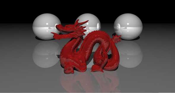
In fact, here was one of the very first images I rendered back in high school with a simple recursive ray tracer written in Java:

I am very fortunate to be a student in Professor Ravi Ramamoorthi’s CSE 168 class at UCSD, where we get to learn about physically-based rendering methods as well as other modern path tracing algorithms. Over the duration of this course, we’ve begin incrementally building up a modern path tracer, starting with a path tracer handling only direct light and adding indirect lighting, next event estimation, Russian Roulette, physically-based GGX BRDFs, and multiple importance sampling features. The path tracer also runs using NVIDIA’s OptiX 6.5 framework, which allowed me to take advantage of my laptop’s GTX 1050 to gain a significant speed improvement.

For my final project in this class, I will be extending the path tracer with the following algorithms:

• Depth of Field Effects
• Texture Mapping
• Glass Microfacet BTDFs
• Smoke via Volumetric Path Tracing

Additionally, I have crafted my own scene to best showcase these new features. Please see below for a description of this process.

Do note that this is still a work in progress (hence the part I). The glass BTDF and volumetric path tracing are currently incomplete.

Creating a Reference Image

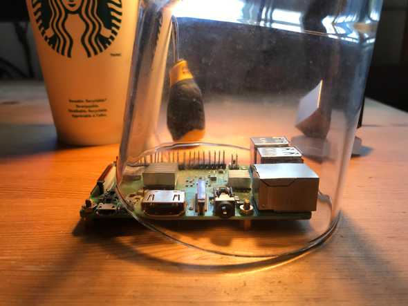
My first step was to create a reference image. I wanted to use objects in my scene that I actually have interacted with on a daily basis to make it more personal. It was also convenient for me to use these objects since they were readily available in my room.

I have specific reasons for using and positioning these objects like so. You can read more in my proposal.

Crafting a 3D Scene using Blender

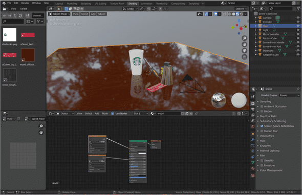
The next step was to recreate this scene using a 3D computer graphics modeling suite. I choose to use Blender, since it works reasonably well on Linux, is free, and comes with many handy features, such as imports/exports to and from a variety of different formats, path tracing and rasterizer previews, and the ability to attach realistic materials to objects in the scene (including specifying their BRDFs).

Before this experience, I had never actually worked with any 3D rendering software, much less an advanced tool like Blender, so it took me a while before I felt comfortable using it. Blender’s learning curve reminds me of that of Vim: it’s difficult to navigate around at first when you don’t know any of the keybindings and tools, but as you learn more and more, you eventually reach a critical point at which it suddenly seems much easier.

In addition to learning Blender, I also spent several hours actually making my scene. There were two challenging parts to this:

1. Finding the models and textures to use. I scoured

a bunch of free sites, such as Sketchpad and Clara, searching for the right, free models. Ideally, I would search for .obj/.mtl or .fbx file formats, since they come with good textures and Blender seems to like them. I should note that I was even unable to find a suitable model for the Raspberry Pi in my original image, so I swapped it out with a microcontroller breadboard.

2. Scaling and positioning all of the models. Importing

them is half the battle. In addition to all of the models, I also set up where my camera and light should be.

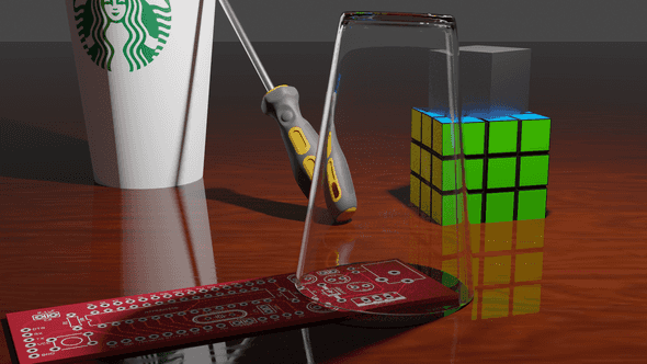
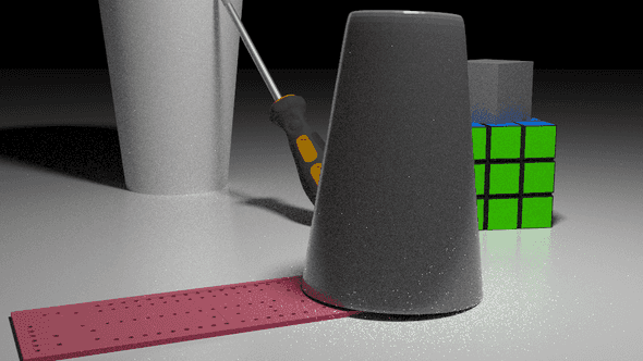
At the end, I found myself with a pretty nice scene. I rendered a preview using Blender’s Cycles engine, which provided me with a benchmark from which I could gauge progress on my own path tracer.

Do note that I didn’t enable any smoke or depth effects when using Cycles, so this image isn’t completely accurate. I also swapped out the wood textures and made the tungsten cube less reflective, so this image is slightly outdated. It’s still a good preview nonetheless.

Importing the Scene into my Path Tracer

At this point, my scene was basically complete. However, I needed some way to transfer the scene out of Blender and into my own path tracer, since my original path tracer was only configured to read specially formatted CSE 168 .test files.

There were several options to choose from:

• .dae “Collada” format: This format was appealing for

many reasons. It’s human readable, it includes camera and lighting data, it has support for “extra” data that can be appended to each object, and it’s Blender’s first choice for exports. However, I ended up not using it because Blender kept distorting the rubber handle on my screwdriver, so when I re-imported it, the mesh looked completely wrong.

• .fbx format: This format is probably the smallest out of

my options because it’s not human readable. It’s also proprietary. Those two issues dissuaded me from using it.

• .obj/.mtl “Wavefront Object/Material” format: This is

the choice I ended up settling on.

The Wavefront object file format is extremely well-known, and there exist many C++ libraries such as BLY-7’s OBJ-Loader that can handle it very well. The object file format has support for texture and shading data. Texture coordinates are kept inside vertices, and links to the texture files are kept inside the material file.

There were two main problems with the Wavefront object file format unfortunately. I had to work around these:

• No camera or lighting data saved. Object file formats describe

objects, not scenes. My workaround was to store this data in a separate .test CSE 168 file. This scene file then referenced my object file to load the objects in the scene. The camera, lighting, and other parameters were kept inside the overarching scene file. I manually copied all of the positions of the camera and the light from my scene; one annoyance with this approach was that Blender keeps its positions in Y-up format (the Y-axis is the up direction) where my path tracer was using Z-up format. In the object file, Blender will automatically convert its Y-up system to a Z-up system, so thankfully, that was all taken care of. But, unfortunately, that conversion had to take place manually for my camera and light; it took me a bit to figure all of that out.

• Object files only support primitive Blinn-Phong shading parameters,

which are non-PB. However, my scene in Blender was using physically-based “principled” microfacet BRDFs in all internal material data. Blender’s solution to this is to encode all of this PBR information into the Blinn-Phong parameters. For example, when Blender exports its BRDF “roughness” parameter, it will turn this into a shininess value in the range of [0, 900] by subtracting the roughness value from 1, multiplying it by 30, and the squaring it. My solution to this problem was just to adapt Blender’s import source code appropriately in my own path tracer.

Rendering the Outline

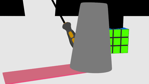
To make sure everything was working, I first disabled all of my shading and recursive path tracing. Instead, whenever I hit an object, I would just return the object’s diffuse color immediately. This allowed me to continually tweak my camera’s parameters until I felt satisfied that I had replicated the original scene in Blender to a reasonable extent.

This left me with the following scene.

It’s not very pretty, but you can see the outlines of all of the different objects, which is exactly what I needed.

Applying Shading

The next step is to add back shading. This served two purposes.

1. I could gauge the position of my light in the scene using the shading

of the objects as reference.

2. I could better tweak my interpretation specular, diffuse, and roughness

parameters until I was satisfied that they looked natural.

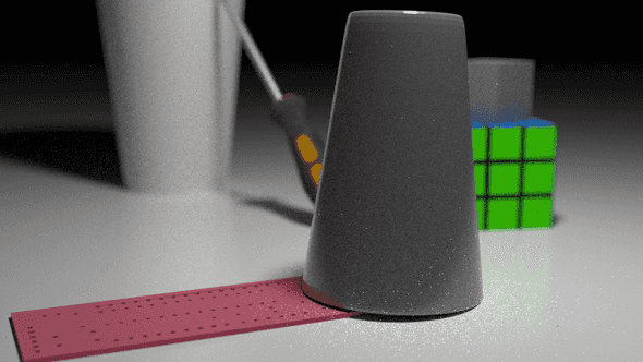
After some fiddling, I managed to get this scene.

Perfect. The materials with no textures, such as the tungsten cube and Rubik’s cube, looked very realistic without much adjustment, owing to the microfacet BRDF implemented previously. For more context on what this BRDF is, please see this paper. The microfacet distribution used is GGX. BRDF importance sampling, next event estimation, and multiple importance sampling were all enabled. 64 samples per pixel were taken. These contants remain the same for all subsequent images.

The Depth of Field Effect

My next step was tackling depth of field. My current path tracer was assuming that a “pinhole” camera model is in use. This means that the camera is treated as a fixed point in space; all camera rays start at the camera’s origin position.

Obviously, this is not physically accurate. In real life, cameras have a lens through which light is captured. Not all light is directed to a single point in the camera. This is what results in depth of field, wherein a camera is able to focus on an object and make the rest of the scene blurry. There are two parameters that control this depth of field effect:

1. Focal distance. The focal distance of a camera specifies how far out

it focuses. For a real camera, this is usually given in terms of millimeters. 2. Aperture size. The aperture size controls the blurriness of the objects not in focus. For a real camera, the aperture is usually specified in an inverted fashion, such that a small aperture usually means an out-of-focus background. A wide aperture, conversely, would indicate that the background is more in-focus.

This effect can be simulated in my path tracer by making a modification to how my camera is set up. I added two additional parameters to describe my camera, focal distance and aperture size. Then, I modified my camera ray generation algorithm as such:

1. Calculate the camera’s origin and outgoing ray direction as one would

in a pinhole camera. 2. Generate a focal point by computing origin + direction * focal length. 3. Generate any perpindicular vector to the outgoing ray direction and normalize it. I did this by taking the cross product of my camera’s up vector and the ray direction and then normalizing the result. This vector I call “offset vector 1”. 4. Generate a third perpindicular vector by taking the cross product of offset vector 1 and the outgoing ray direction. I call this vector “offset vector 2”. 5. Now, generate a random float between [-0.5, 0.5] and multiply it by the aperture size. Then, scale “offset vector 1” by this random float. 6. Do the same for “offset vector 2”. 7. Add both offset vector 1 and offset vector 2 to the camera origin. This is the new origin of the outgoing ray. 8. Finally, generate a new outgoing direction by subtracting the focal point from the new origin and normalizing the subtraction.

This algorithm effectively simulates an aperture. The ray’s origins are perturbed such that they could be anywhere in the aperture circle that is perpindicular to the direction the camera is facing. If the aperture size is set to a very large number, then the simulated aperture will be very large and you will get rays that start at a completely different distance from the origin of the camera. If the aperture is small, the camera ray’s origins will be very close to the original camera position. If the aperture is 0, then you effectively have a pinhole camera again.

I set my camera to focus on the glass cup and use a big-enough aperture size to produce visibly distinct blurring.

Texture Mapping

Next up is texture mapping. When implementing texture mapping, I disabled my depth of field effect temporarily so that I could verify that my textures were appearing correctly on my background objects.

Textures are very well understood in the realm of computer graphics, and there exist many different types of texture mappings, for example, roughness maps, normal maps, diffuse maps, and displacement maps. For this project, I wanted to focus on diffuse maps, that is, images that take the place of the diffuse color of the object.

When Blender exports a scene as a Wavefront object file, it encodes two parameters into the resultant object and material files that are necessary for texture mapping.

1. In the object file, each vertex has a texture coordinate added to it.

A texture coordinate (u, v) describes where that vertex maps to in the texture image (more on this later). Note that vertices only have texture coordinates if their corresponding mesh material has a mapped image. 2. In the material file, the map_Kd <FILE> parameter specifies that a material has a diffuse texture map (hence the Kd) located at the file found at <FILE>.

Because textures are so commonplace, NVIDIA’s OptiX framework piggy-backs off of CUDA’s own support for OpenGL textures and adds additional parameters specifying mipmap levels, read modes, and more. Most importantly, they provide support for reading an image at a specific texture coordinate, essentially abstracting away much of the math (behind the scenes, I set my texture sampler to linearly interpolate between pixels). This simplifies the texture mapping process greatly, effectively reducing it to this process:

1. Read the image into a GPU buffer that OptiX can pass to my CUDA shader.
2. Attach this GPU buffer to an OptiX texture sampler object, which then yields

an immutable device ID that can be used to query the sampler. 3. Store this device ID in a separate GPU buffer. Store the device ID’s index in this buffer in each of the mesh’s triangles. 4. Repeat steps 1-3 for all textures. 5. Inside the shader, in the intersection program, calculate texture coordinates at a triangle hit point. Look up the device ID using the triangle’s device index and then use index into the associated texture sampler using the texture coordinate to produce a diffuse color.

Steps 1-4 can be accomplished by reading the OptiX documentation (specifically, the texture section 3.3). Step 5 is a bit more tricky.

To get step 5 to work, it’s important to first understand briefly what barycentric coordinates are. Barycentric coordinates are the product of a special coordinate system that essentially assigns uniquely a triplet of numbers to every point in the area of the triangle. This triplet has the special property that the sum of its components is 1. Whenever we intersect a ray with a triangle, we can calculate the barycentric coordinates of the intersection point. But how does this relate to texture mapping?

The texture mapping process described in steps 1-4 assigns every vertex in every triangle a unique pair of coordinates, referred to as texture coordinates. A texture coordinate uniquely maps to a point on the image, much like a barycentric coordinate uniquely maps to a point on a triangle.

When we calculate the barycentric coordinates of an intersection point, we also have available the texture coordinates of each of the triangle’s 3 vertices. We can then use the barycentric coordinates (u, v, 1 - u - v) to linearly interpolate between the 3 texture coordinates to produce a new texture coordinate. This new texture coordinate can then be looked up in the image with this part being handled by OptiX.

Let’s try this out.

Wait … these textures look off! Even though the textures are associating correctly with each object, they aren’t being mapped properly, which is producing weird jagged lines of diffuse color.

It must be an issue with the barycentric coordinates then. The barycentric coordinates I am generating have been well tested in the Moller-Trumbore intersection algorithm I have been using for triangles. Therefore, it must be an issue with my interpolation.

Indeed, permuting the barycentric coordinates in the correct fashion yields the correct image.

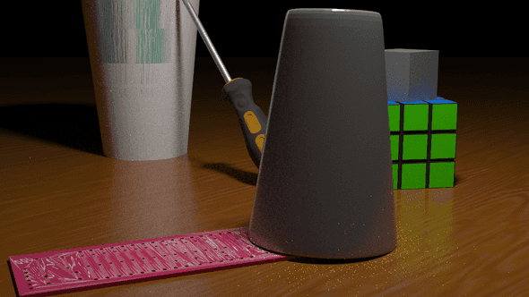
Now that textures are working properly, I can combine it with the depth of field effect to produce a crisp render.

What’s Next?

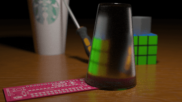
The next steps for me are implementing the refractive BTDF described in the microfacet BSDF paper listed above. The glass cup is assumed to be made out of Flint glass, with an index of refraction of 1.51. In contrast, air has an index of refraction of 1.003.

This BTDF isn’t fully finished yet. There are a lot of tweaks that need to be made to the sampling procedure before it is ready, as well as possibly to the evaluation and PDF functions. As you can see in the glass, the transmission is oddly mirrored, which is likely the result of an incorrect refraction implementation. I am still actively looking into this.

I’m hoping to have a basic form of volumetric path tracing implementing after the glass BTDF is wrapped up, at which point my scene will be fully complete.

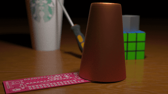
In meantime, here’s the scene rendered with a bronze cup instead of a glass cup!